Definition of wiki : The Java collections framework (JCF) is a set of classes and interfaces that implement commonly reusable collection data structures.

The above diagram contains the common implementation of collection framework

The above diagram contains the common implementation of Map.
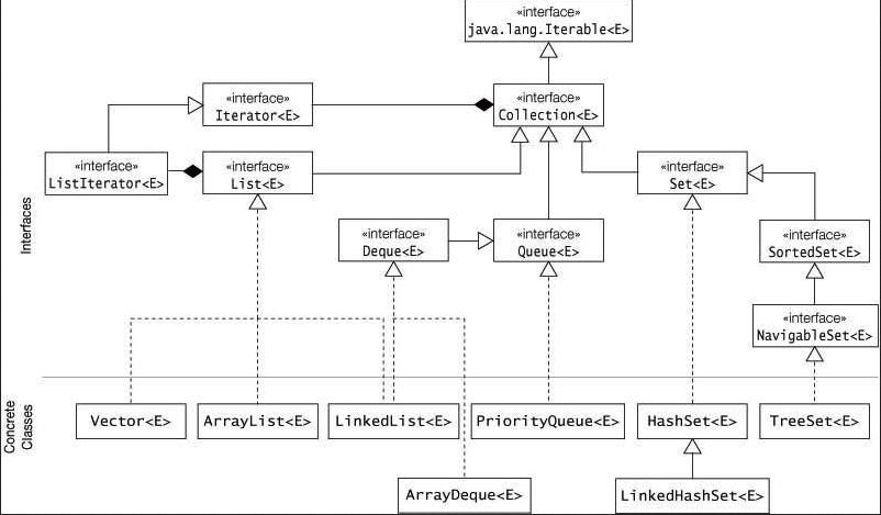
The above diagram contains the common implementation of collection framework

The above diagram contains the common implementation of Map.
| Concrete Collection/Map | Interface | Duplicates | Ordered/Sorted | Methods That Can Be Called On Elements | Data Structures on Which Implementation Is Based |
|---|---|---|---|---|---|
| HashSet<E> | Set<E> | Unique elements | No order | equals() hashCode() | Hash table and linked list |
| LinkedHashSet<E> | Set<E> | Unique elements | Insertion order | equals() hashCode() | Hash table and doubly-linked list |
| TreeSet<E> | Sorted-Set<E> NavigableSet<E> | Unique elements | Sorted | compareTo() | Balanced tree |
| ArrayList<E> | List<E> | Allowed | Insertion order | equals() | Resizable array |
| LinkedList<E > | List<E> Queue<E> Deque<E> | Allowed | Insertion/priority/deque order | equals() compareTo() | Linked list |
| Vector<E> | List<E> | Allowed | Insertion order | equals() | Resizable array |
| PriorityQueue<E> | Queue<E> | Allowed | Access according to priority order | compareTo() | Priority heap (tree-like structure) |
| ArrayDeque<E> | Queue<E> Deque<E> | Allowed | Access according to either FIFO or LIFO processing order | equals() | Resizable array |
| HashMap<K,v> | Map<K,V> | Unique keys | No order | equals() hashCode() | Hash table using array |
| LinkedHashMap<K,V> | Map<K,V> | Unique keys | Key insertion order/Access order of entries | equals() hashCode() | Hash table and doubly-linked list |
| Hashtable<K,V> | Map<K,V> | Unique keys | No order | equals() hashCode() | Hash table |
| TreeMap<K,V> | Sorted-Map<K,V> NavigableMap<K,V> | Unique keys | Sorted in key order | equals() compareTo() | Balanced tree |
List Interface.
An ordered collection.
- The user of this interface has precise control over where in the list each element is inserted.
- The user can access elements by their integer index (position in the list), and search for elements in the list.
1. Search for a specified object
2. Remove and insert elements at an arbitrary point in the list.
Key implementations of List interface
1. ArrayList<E>: A list implementation with underlying data structure is arrays.
- Implements all optional list operations,
- permits all elements, including null.
- The size, isEmpty, get, set, iterator, and listIterator operations run in constant time.
- Adding n elements requires O(n) time. An application can increase the capacity of an ArrayList instance before adding a large number of elements using the ensureCapacity operation. In ensureCapacity operation. if additional element increases the old capacity of array list then. Arrays are copied into new ArrayList with size = (oldCapacity * 3)/2 + 1
1. Add (E e): Increase capacity if required and then add the element at the last in a new Array
2. Add(int index, E e) : Increase the capacity if required , then use System.arrayCopy to copy except the index postion
3. Remove(int index) : use System.arrayCopy to shifts any subsequent elements to the left
4. Remove(E e) : iterates over the array and removes the first element that matches in the array.
ArrayList provides random access and is more efficient at accessing elements but is generally slower at inserting and deleting elements.
2. LinkedList<E>: A doubly linked list implementation.
- Implements all optional list operations,
- permits all elements, including null.
- The size, isEmpty, get, set, iterator, and listIterator operations run in constant time.
- Insert operation is fast as you just have to change the pointers of the linked list instead of copying the whole array.
- This data structure to be used when we frequently add and remove elements from the list.
1. get(index) : Iterates over the list to get element.
2. Add (E e): Append the element at the end of the list
3. Add(int index, E e) : get the element at the index position and then set the object at that index
4. Remove(int index) : get the element at the index position and then set remove the object references.
5. Remove(E e) : Removes the first occurrence of the specified element from the list.
LinkedList provides sequential access and is generally more efficient at inserting and deleting elements in the list, however, it is it less efficient at accessing elements in a list.
Map<K,V> Interface.An object that maps keys to values. A map cannot contain duplicate keys; each key can map to at most one value.
Interface provide contract for various methods like
1. Search for a specified object based on key
2. Get and put elements based on keys.
Key implementations of Map interface
1. HashMap<K,V>: A map implementation with underlying data structure a array of linked lists.
- Implements all optional map operations,
- permits key and value as null.
- This implementation provides constant-time performance for the basic operations (get and put),.
- An instance of HashMap has two parameters that affect its performance: initial capacity and load factor. The capacity is the number of buckets in the hash table, and the initial capacity is simply the capacity at the time the hash table is created. The load factor is a measure of how full the hash table is allowed to get before its capacity is automatically increased. When the number of entries in the hash table exceeds the product of the load factor and the current capacity, the hash table is rehashed (that is, internal data structures are rebuilt) so that the hash table has approximately twice the number of buckets.
- threshold is DEFAULT_INITIAL_CAPACITY * DEFAULT_LOAD_FACTOR
1. get (k key):
- hash the key : int hash = hash(key.hashCode());
- get the index of linked list array based on hash key and table length
- Iterate over the linked list at that index till key with same reference or equal value is not found
- hash the key : int hash = hash(key.hashCode());
- get the index of linked list array based on hash key and table length
- Iterate over the linked list at that index till key with same reference or equal value is not found and replace the old value
- If the key does not exist then create a new entry at index calculated in step 2 and then re-size the table of linked list

HashMap are efficient for locating a value based on a key and inserting and deleting values based on a key.
2. LinkedHashmap<E>: A doubly linked list implementation.
3. TreeMap<E> : A Red-Black tree based
NavigableMap implementation.
The map is sorted according to the natural
ordering of its keys, or by a Comparator provided at map
creation time, depending on which constructor is used.
This implementation provides guaranteed log(n) time cost for the containsKey, get, put and remove operations.
TreeMap performs all key comparisons using its compareTo (or compare) method, so two keys that are deemed equal by this method are, from the standpoint of the sorted map, equal.
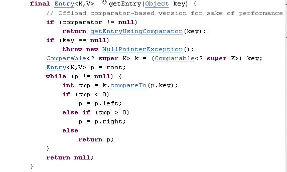
According to the API documentation the Treemap is a red-black tree. Please refer this to understand more.
Set<E> Interface.
A collection that contains no duplicate elements. More formally, sets
contain no pair of elements e1 and e2 such that
e1.equals(e2), and at most one null element.1. Great care must be exercised if mutable objects are used as set elements.
Key implementations of Setinterface
1. HashSet <E>: This class implements the Set interface, backed by a hash table (actually a HashMap instance). It makes no guarantees as to the iteration order of the set; in particular, it does not guarantee that the order will remain constant over time. This class permits the null element.
- Implements all optional set operations, underlying data structure is Hash Map.
- permits null but only one null value.
- This class offers constant time performance for the basic operations (add, remove, contains and size), assuming the hash function disperses the elements properly among the buckets
- Iterating over this set requires time proportional to the sum of the HashSet instance's size (the number of elements) plus the "capacity" of the backing HashMap instance (the number of buckets). Thus, it's very important not to set the initial capacity too high (or the load factor too low) if iteration performance is important.

2. LinkedHashSet<E>: A LinkedHashSet is an ordered version of HashSet that
maintains a doubly-linked List across all elements. Use this class instead of HashSet
when you care about the iteration order. When you iterate through a HashSet the
order is unpredictable, while a LinkedHashSet lets you iterate through the elements
in the order in which they were inserted. Does not have any implementation method extend all methods from HashSet<E>
3. TreeSet<E> : A
NavigableSet implementation based on a TreeMap.
The elements are ordered using their natural
ordering, or by a Comparator provided at set creation
time, depending on which constructor is used.This implementation provides guaranteed log(n) time cost for the basic operations (
add, remove and contains).